Understanding Instantaneous Power Through Python and Physics
Written on
Chapter 1: Introduction to Instantaneous Power
In this article, we delve into the concept of instantaneous power in physics, specifically in the context of mechanical work. Drawing from the textbook "Advanced Physics Demystified" (Gibiliseo 2007), we will explore a problem related to calculating instantaneous power from a function that predicts work over time. The aim is to develop a clearer understanding of mechanical power, benefiting students and enthusiasts alike.
The question posed is:
“Given a function for mechanical work over time (Eq. 1), where work ( w(t) ) is expressed in newton-meters and time ( t ) in seconds, how can we determine the instantaneous power at ( t=3 ) seconds?” — A paraphrased version of Gibiliseo's inquiry.

Eq. 1.1
Before we tackle the solution, it's essential to grasp what “instantaneous power” entails.
What is "Power"?
In a political framework, power signifies the capacity to influence outcomes and control circumstances through social interactions (Barnett & Duvall 2005). While this definition pertains to social sciences, it can serve as an analogy for understanding mechanical power in physics. In this context, power refers to the rate at which a mechanical force influences the displacement of an object.
The analogy between political and mechanical power, although insightful, has its boundaries due to the differing methodologies of analysis in the two fields (Kellstedt & Whitten 2013; Taleb 1996).
Formal Definition
In our scenario, we are examining instantaneous power as a function of time. Let ( t ) represent time and ( w(t) ) denote the total work performed. Instantaneous power ( P ) is formally defined as:

Eq. 1.3
To visualize mechanical work, I will plot the ( w(t) ) function on a Cartesian graph. This will be accomplished using the JupyterLab application (Bektas 2021) and Python (n.d.) for creating the chart.
First, I will import necessary libraries and configure the graph:
%matplotlib inline
import math
import sympy
import numpy as np
import matplotlib.pyplot as plt
plt.figure()
plt.rcParams["xtick.bottom"] = plt.rcParams["xtick.labelbottom"] = False
plt.rcParams["xtick.top"] = plt.rcParams["xtick.labeltop"] = True
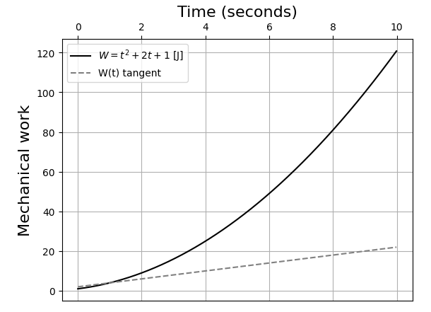
Next, I will compute the derivative of Eq. 1.1 to illustrate the relationship between instantaneous power and mechanical work. The derivative in this case is ( 2t + 2 ). Here’s the Python code to create a plot showing time against Eq. 1.1 and its tangent line:
wt_function = lambda t: t**2 + 2*t + 1
dwt_function = lambda t: 2*t + 2
range_t = np.arange(0, 10, 0.01)
plt.figure()
plt.plot(range_t, [wt_function(t) for t in range_t], color="black", label=r'$W = t^2 + 2t + 1$ [J]')
plt.plot(range_t, [dwt_function(t) for t in range_t], "--", color="grey", label="W(t) tangent")
plt.grid()
plt.legend()
plt.title("Time (seconds)", fontsize=16)
plt.ylabel("Mechanical work", fontsize=16)
plt.show()
Figure 1 displays the outcomes of the code:

Figure 1: Mechanical Work Visualization
Unit Derivations
To better understand the physics involved, we will derive fundamental units such as newtons and velocity measures, allowing for calculations and potential verification of results.
Velocity is defined as meters per second:

Eq. 1.2.1
Acceleration is expressed in meters per second squared:

Eq. 1.2.2
Mechanical force, as per Newton's second law, is calculated in kilograms multiplied by the acceleration value:

Eq. 1.2.3
Mechanical work is quantified in joules, defined through its respective equation:

Eq. 1.2.4
Finally, mechanical power, measured in watts, can be defined as follows:

Eq. 1.2.5
With this foundational knowledge established, we can now proceed to the solution.
Chapter 2: Solution Methodology
The derivative calculated in the previous section illustrates the relationship between instantaneous power and mechanical work. However, it is essential to verify this derivative through both calculus and computer algebra.
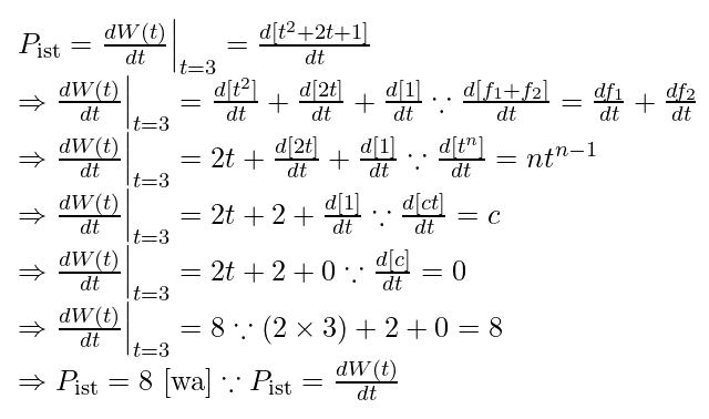
The derivative for Eq. 1.1 can be computed using calculus as shown:

Eq. 2.1
To confirm this result, I utilized the SymPy computer algebra system within JupyterLab. The following code allows me to check my work:
w, t = sympy.symbols("w t")
w = t**2 + 2*t + 1
p_inst = sympy.diff(w, t)
display (p_inst)
The outcome of this process is depicted in Eq. 2.2:

Eq. 2.2
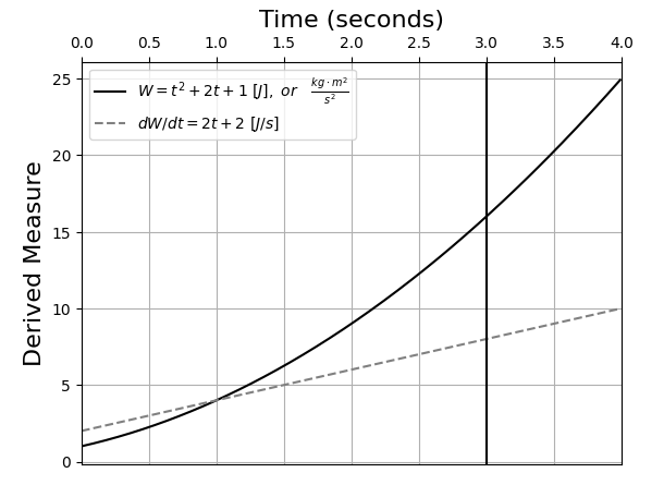
Substituting ( t = 3 ) into this equation yields a result of ( 8 ) watts. This confirms the correctness of both my manual and computer-derived solutions. To visualize this solution and the disparity between the mechanical work function and its corresponding instantaneous power at ( t=3 ) seconds, I generated a chart (figure 2) similar to figure 1:

Figure 2: Comparing Mechanical Work and Instantaneous Power
The following Python code was used to create figure 3:
wt_function = lambda t: t**2 + 2*t + 1
dwt_function = lambda t: 2*t + 2
range_t = np.arange(0, 4, 0.01)
plt.figure()
plt.plot(range_t, [wt_function(t) for t in range_t], color="black", label=r'$W = t^2 + 2t + 1 [J], or frac{kg cdot m^2}{s^2}$')
plt.plot(range_t, [dwt_function(t) for t in range_t], "--", color="grey", label=r'$dW/dt = 2t + 2 [J/s]$')
plt.axvline(x = 3, color="black")
plt.grid()
plt.legend()
plt.title("Time (seconds)", fontsize=16)
plt.ylabel("Derived Measure", fontsize=16)
plt.xlim(0, 4)
plt.show()
Allora.
End Matter
Through this discussion, I aimed to clarify a fundamental physics problem related to mechanical power and develop an intuitive understanding of the concept. However, as a learner myself, I advise readers to seek authoritative texts or professionals for a deeper exploration of mechanical power.
Acknowledgements
I would like to express my gratitude to Saha (2015) for their insightful work on applying Python to scientific computing, which greatly aided in coding for this project.
References
Gibiliseo, S. (2007). Advanced Physics Demystified [Paperback]. McGraw-Hill Education.
Kellstedt, P. M. & Whitten, G. D. (2013). The Fundamentals of Political Science Research. Cambridge University Press.
Saha, A. (2015). Doing Math with Python: Use Programming to Explore Algebra, Statistics, Calculus, and More! No Starch Press.
Taleb, N. N. (1996). Dynamic Hedging: Managing Vanilla and Exotic Options. John Wiley & Sons.
Level Up Coding
Thank you for being part of our community! Before you leave, feel free to clap for the story and follow the author. Explore more content in the Level Up Coding publication. Check out our free coding interview course and follow us on Twitter, LinkedIn, and our Newsletter. Join the Level Up talent collective to find an amazing job!